Following our previous experiment, the logical step is to create something slightly more complex using the logistic regression algorithm we have built. To do so, we will expand the “hidden units” or “hidden layers” in our network, which is to say that we will add stages to our forward propagation.
Ok but why?
Given the data set we used in the previous tutorial, linear regression was enough since the input data presented a problem solvable by a linear process. Nevertheless, when the problem is non-linear, we will see that logistic regression alone is not enough. We need to add hidden units to get better results, along with some tweaking of parameters.
Ours will be a model where we have two hidden units to compute our learning process. Some problems in Machine Learning require “deep” neural networks, while others will do fine with “shallow” models. A 5-hidden layers model is somewhat “deep”, while a one or 2-hidden layer model is “shallow”. In the case of this example, we will build a network with one input layer (the training examples), one hidden layer (our neurons), and one output layer.
For our experiment with this “shallow” classifier, I use the make_moons() toy data set, offered in Python’s sklearn library, whose solution is non-linear.
Generating the dataset
To get our targeted data-set, we can run the following code from a Python interpreter:
# Generate some data
#____________________
from sklearn import datasets
import matplotlib.pyplot as plt
# Get 10 points from the make moons data set
# We set the random state to 0, so we have reproducible data
X, y = datasets.make_moons(10, random_state=0, noise=0.0)
# Write data to a file
with open('moons_dataset.txt', 'w') as f:
	f.write('{}{}{}'.format('x', 'y', 'class'))
	for i, coord in enumerate(X):
	    f.write('{}{}{}'.format(coord[0], coord[1], y[i]))
#Plot the data
plt.figure(figsize=(8, 8))
plt.scatter(X[:, 0], X[:, 1], marker='o', c=y, s=25, edgecolor='k')
plt.show()
The code will generate a file called “moons_dataset.txt” that we can then import into TouchDesigner and convert to a table for our experiment.
Note: If you can run sklearn from within TouchDesigner, it is easy to adapt the script to create a table directly with this data. As of writing this tutorial, some people have experienced issues importing modules that do not come with the native Python version (3.5) in TouchDesigner (TD) due to some conflicting library invocations that occur when a newer Python version exists. If that happens, this code will help you generate data that you can import from outside TD.
The data set looks like this, where the red dots represent a class 1 and the blue ones a class 0:

The goal
The solution for this data set is non-linear, and it looks like this:

Our goal in the coming tutorials is to build a shader consisting of a shallow two-layered neural network with 3 to 5 neurons that can find this solution. Given how shaders work, we will see that this is not so straightforward to do, so as we said, let us go step by step and build first this shallow network with a single neuron in its hidden layer, to understand how we can think about this.
Expressing the problem
Our setup for the input data does not differ much from what we have built in the previous experiment. We set the data in the same way, except that in this case, we are using the dataset we have generated with the help of sklearn, which I am importing from an external file.

You could build a simple visualizer using instancing as a helper to make sure your data is correct. One such visualizer is offered here in a .tox for you.
The math
In addition to the equations we have seen before, we need to create further steps since we are dealing with an extra hidden layer. So, where before we had weight $w$ and bias $b$, now we need to account for our extra hidden layer: $w_1$, $w_2$ and $b_1$, $b_2$. Similarly, we are going to have two steps of derivatives in our backward propagation: $dw_1$, $dw_2$ and $db_1$, $db_2$. Our general algorithm to compute all of these would be (assuming operations with matrices, represented by capital letters):
$m = samples$
Our hidden layer:
$Z_1 = W_1X + b_1$
$A_1 = g_1(Z_1)$
Output layer:
$Z_2 = W_2A_1 + b_2$
$hat{y} = A_2 = g_2(Z_2)$
Where $g$ is the activation function at each step. We use the notation $A$ to denote the output of the activated weight from an operation. As you can see, this is simply stacking the operations one after the other:
- $Z_1$ is the intermediate output of the hidden layer.
- $A_1$ is the activated output of the hidden layer.
- $Z_2$ is the intermediate output of the output layer.
- $A_2$ is the final activated output of the network.
In this case, we will use a $tanh$ activation function for the hidden layer, and a sigmoid function for the output layer, since we are building a classifier.
Activation functions
If you are not sure why we use first a tanh and then a sigmoid function, you may understand it as a tool to map the data to ranges that are useful for the classification process.
These functions are responsible for “firing” a neuron since they tell the algorithm whether a neuron is significant in the learning process or not. Depending on the problem and the stage, we want to use different activation functions, so that the weights get mapped to a proper range.
The tanh or “hyperbolic tangent” function looks like this:
We use this as the first step in the forward propagation stage. When a value passes this function, after bipolar random initialization, it can quickly move upwards or downwards because of its vertical bipolar range and the steepness of the curve between (-1.0, 1.0) along the x-axis.
It is not the only option, as we will see later. It may not even perform as well as another activation function called RELU for this problem. However, we are using it here because it is more intuitive to understand than other alternatives.
Later on, at the last stage of our algorithm, we will employ the sigmoid function, which looks very similar to the tanh but is in the range (0, 1). That makes it ideal for classification because it can tell us what probability a given class has, given that the range is finite and is normalized.
This explanation is simplistic, but it is sufficient for us now. If you want to dive into it more deeply, I suggest reading this excellent article by Avinash Sharma V, which explains activation functions in an informal, yet transparent way.
Proceeding with the math
Alright, now to compute cost, we use logistic regression with cross-entropy:
$-frac{1}{m}sum_{i=1}^{m}[Y logA_2 + (1-Y)log(1-A2)] $
Notice that this expression has the negative mean of the sum of the whole set of losses:
$-1/m * sum(losses)$
or
$-sum(losses)/m$
For the back-propagation:
$dZ_2 = A_2 – Y$
$dW_2 = frac{1}{m} dZ_2 A_1^T$
$db_2 = frac{1}{m} sum_{i=1}^{m}[dZ_2]$
We now have to compute the derivatives of the activation functions, for the first layer:
$gprime = {g}'(Z_1)$
Derivatives of our first hidden layer:
$dW_1 = frac{1}{m} dZ_2 X^T$
$db_1 = frac{1}{m} sum_{i=1}^{m}[dZ_1]$
And finally to update our parameters:
$W_1 = W_1 – alpha dW_1$
$b_1 = b_1 – alpha db_1$
$W_2 = W_2 – alpha dW_2$
$b_2 = b_2 – alpha db_2$
Implementation
Like before, we want to output a single pixel for the computation so that everything runs only once in the shader, meaning that our resulting shader will output a resolution of 1×1. Notice that now we need to output 2 textures from the shader, since we have two distinct set of values for $w_1, b_1$ and $w_2, b_2$.
How can we achieve this?
One way to do this is to make use of TouchDesigner’s “#color buffers” option. In this manner, we can write a texture for each of our hidden layers. If you are not familiar with this concept, you may want to check out this resource: color buffers (jump to the “Outputting to Multiple Color Buffers” section). We will use a GLSLmulti TOP for this endeavor since it allows us to input more than three textures at once.
In the shader, write the following code to initialize our color buffers and our uniforms: (don’t forget to increase the # of color buffers parameters in the preferences of the GLSL TOP to 2)
uniform int numExamples;
uniform int uReset;
uniform float learningrate;
layout(location = 0) out vec4 weights1;
layout(location = 1) out vec4 weights2;
Next, we create helper functions for the sigmoid activation function and a pseudo-random number generator, given that in a neural network we have to initialize the values for our weight and biases randomly, so that they can move somewhere:
float random(vec2 st, float seed) {
	return fract(sin(dot(st, vec2(15.63547, 87.84849))) * seed);
}
float sigmoid(float z) {
	return 1.0 / (1.0 + exp(-z));
}
Now, the most important part: getting the matrix dimensions right. It is so crucial that we will devote a whole chapter just to that. Let us have a first look.
Matrix dimensions
In my explorations with Deep Learning, this seems to be by far the most important thing to learn how to do. Once you get matrix dimensions right and have understood why it has to be the way it is, then all the rest starts falling in place.
When jumping from Python implementation using NumPy, or a library like TensorFlow to this GLSL experiments in shaders, things can be confusing because computations always run parallely. We have so far dealt only with vectors instead of thinking directly in matrix operations.
Don’t worry. We will progress to make life easier for ourselves in the coming tutorials using matrix multiplication instead. The first thing to understand is: how does matrix multiplication work in terms of dimensions? Here is the intuition with a drawing from Coolmath:
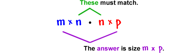
We can see how to make sense of things further down the line of our implementation. The simplest and best way to know the dimensions of the respective matrices for computation is to go and draw the data graph we are modeling. Remember that in this example, we are dealing with vectors, which are uni-dimensional matrices, so the principle still applies!
Here is a diagram with a cheat technique to calculate the dimensions of each element in our Neural Network (NN) using the above intuition. Take a moment to carefully analyze what is going on:

We can tell the dimensions we are expecting for each corresponding element in every step of our computation.
With this knowledge, let us initialize our values, assuming we are going to pass these in textures, each of one single pixel:
vec2 uv = vUV.st;
// Initialize
float m = float(numExamples);
float cost = 0.0;
// Gather Weight 1 values
vec3 parameters1 = texelFetch(sTD2DInputs[2], ivec2(0, 0), 0).xyz;
vec2 w1 = parameters1.xy; // a vec2 (1, 2)
float b1 = parameters1.z; // a float (1)
// Gather Weight 2 values
vec2 parameters2 = texelFetch(sTD2DInputs[3], ivec2(0, 0), 0).xy;
float w2 = parameters2.x; // a float (1, 1)
float b2 = parameters2.y; // a float (1)
That may be a little bit confusing. Remember that we can use a vec2 to represent either a (2,1) or a (1,2) matrix, since when dealing purely with uni-dimensional matrices (vectors) where the order doesn’t matter. That would not be true if we were operating between a multi-dimensional matrix and a vector. It works only in this context.
Building up
Like before, we will create a reset check to re-initialize our values when desired and variables to store our forward and backward propagation. Notice the dimensions of the vectors, which are just right to hold the intended data in pixels. The random initializations occur here, hence the funky-looking numbers in the random function. These are a kind of seeds for the pseudo-random number generator. They can be of any value.
if(uReset == 1) {
	float constant = 0.01;
	// Dimensions: w1 =(2, 1), b1 = scalar, w2 = (1, 1) b2 = scalar
	w1 = vec2(random(uv, 11.12), random(uv, 76.33)) * constant;
	b1 = 0.0;
	w2 = float(random(uv, 87.44)) * constant;
	b2 = 0.0;
}
// Store our derivatives in pixels
vec3 derivatives1 = vec3(0.0); // red green = w1 b = b
vec2 derivatives2 = vec2(0.0); // r = w2, g = b
Confused? Good. I’m confused myself again trying to explain this in text.

Oh, wait. Ok, got it! Where were we?
Luckily for us, the rest is pretty straightforward. It is just a matter of setting the equations we already know in a very similar fashion to when we implemented logistic regression with a single neuron.
Forward and backward propagation
// Gather all our input examples
for(int i = 0; i < numExamples; i++) {
	vec2 x = texelFetch(sTD2DInputs[0], ivec2(i, 0), 0).xy; //data
	float y = texelFetch(sTD2DInputs[1], ivec2(i, 0), 0).x; // class
	/////////////////////////// Forward propagation////////////////////////
	// Hidden layer
	float z1 = dot(w1, x) + b1;
	float a1 = tanh(z1);
	// Output layer
	float z2 = w2 * a1 + b2;
	float a2 = sigmoid(z2);
	/////////////////////////// Compute cost////////////////////////
	float logprobs = (y * log(a2)) + ((1.0 - y) * log(1.0-a2));
	logprobs = -logprobs / m;
        cost += logprobs;
	/////////////////////////// Backward propagation////////////////////////
	// Output layerfloat
	dz2 = a2 - y;
	float dw2 = dz2 * a1 / m;
	float db2 = dz2 / m;
	derivatives2 += vec2(dw2, db2);
	// Hidden layer
	float gprime = (1 - pow(a1, 2));
	// tanh derivative
	float dz1 = w2 * dz2 * gprime;
	vec2 dw1 = dz1 * x / m;
	float db1 = dz1 / m;
	derivatives1 += vec3(dw1, db1);
}
And then just update the parameters:
// Update parameters
w1 = w1 - learningrate*derivatives1.xy;
b1 = b1 - learningrate*derivatives1.y;
w2 = w2 - learningrate*derivatives2.x;
b2 = b2 - learningrate*derivatives2.y;
Remember that we said we would output this parameter in two different color buffers and declared at the top of the shader two different output layouts? We are going to use the current shader output for parameters1 (containing $w_1, b_1, cost$ and a second buffer for parameters2 ($w_2, b2_2$)
weights1 = vec4(w1, b1, cost);
weights2 = vec4(w2, b2, 0.0, 0.0);
Alright! We completed the shader. The only thing we are missing is a loop. Like before, we will use feedback to iterate over our data and make the machine learn!
Feedback

As you can see, our approach is the same as in the previous tutorial. The only difference is that now we have two feedback TOPs. One of these uses a Render Select TOP as input since that TOP is grabbing the second color buffer we are emitting from the shader. The other one fetches the texture we are outputting from the shader itself.
Proceed with hooking up the prediction shader we used before and inspect the cost. You should see it coming down, which means that our margin of error is decreasing. In other words, TouchDesigner is learning!

Great job! You can find the full project here including the .tox file, the data-set and the script to generate the dataset.
But hold on. You will see that it is not fully succeeding in predicting the correct classes for each training example. What gives? Maybe our model is not robust enough to solve this accurately, so we will need to refine it to model things accurately.
What if we add more neurons?
Our goal was to solve a non-linear equation, but our cost cannot go down lower than about 0.45 with this implementation. To improve this issue, we will need to create more neurons. As hinted previously, this is a tricky business with shaders, because of the limited data structures we have available.
To understand our difficulty, here is a clarification of why this is not easy to do in the current implementation: if we draw again and observe the graph for our model, this time considering 3 neurons for the hidden layer instead of two, we have:

You can see that $w_1$ needs to be a (3,2) matrix. How exactly would we represent this with vectors? We cannot. We could use a mat3x2, but then that does not solve our problem when we would like to build a matrix with ten neurons, because that data structure does not exist. We could create a custom struct, but that would mean that the matrix multiplication will occur every time we run our loop to iterate over the examples. With ten, that is ten times matrix dimensions of processing per frame. Not exactly efficient!
It is better to find a solution that can scale up, is simple to grasp, and is relatively fast to perform. If only we could have a matrix operator in TouchDesigner…
But wait! We do have it. We have tables, don’t we? These are in fact matrices, but how do we use those in a shader? We could convert them to TOPs. Oh, but then a texture is already a matrix, isn’t it?
So, we could use a texture as a matrix to perform our operation, in a way that makes sense using shaders and that takes full advantage of their parallelism.
In the following tutorial, we will create our matrix multiplication shader. First, to understand deeply how matrix multiplication works, and second to scale up our deep learning experiments with shaders. Let’s go!